Income Consumption Curve Short Note

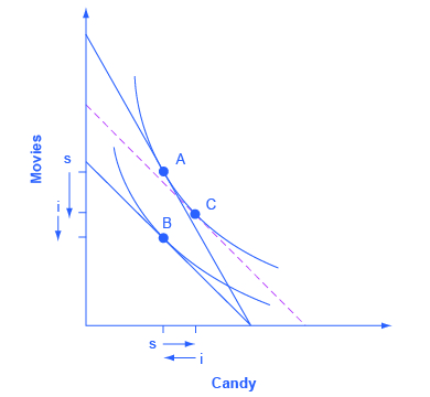
However if the consumer has different preferences he has the option to choose x 0 or x on budget line b2.

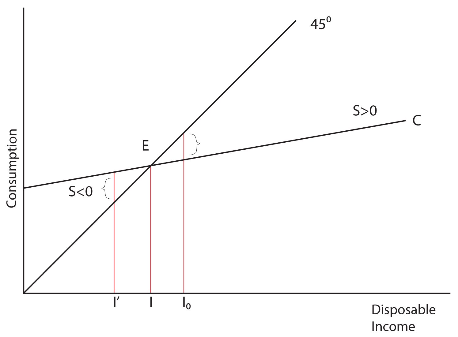
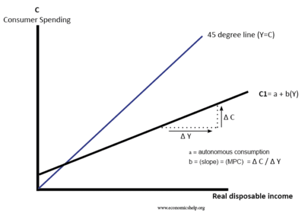
Income consumption curve short note. The figure first shows that the neutral good is measured on x axis or in our case good x is neutral good. Beyond this with the increase in income consumption increases but less than the increase in income and therefore consumption function curve cc lies below the 45 line oz beyond y 0. In the case illustrated with the help of figure 1 both x 1 and x 2 are normal goods in which case the demand for the good increases as money income rises. It is plotted by connecting the points at which budget line corresponding to each income level touches the relevant highest indifference curve.

Also the price effect for x 2 is positive while it is negative for x 1. For instance in fig. Food income 10 2 6 20 100 10 2 8 35 150 10 2 11 45 200 10 2 15 50 250 the income consumption curve connects each of the four optimal bundles given in the table above. 8 33 when income is initially rs.

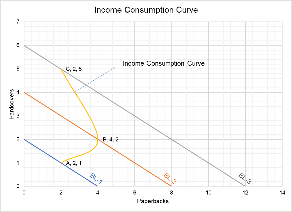
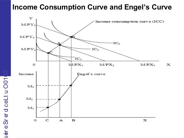
It is thus locus of combinations of the two commodities when the money income is varied and prices of the. The curve obtained by connecting successive consumer s equilibrium points e 1 e 2 and e 3 in this case at various levels of money income of the consumer other things remaining unchanged is known as income consumption curve. For each level of income m there will. The income consumption curve in this case is negatively sloped and the income elasticity of demand will be negative.

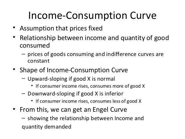
Income consumption curve traces out the income effect on the quantity consumed of the goods. In figure 3 the income consumption curve bends back on itself as with an increase income the consumer demands more of x 2 and less of x 1. Sometimes it is called the income offer curve or the income expansion path. 300 m 1 per week the quantity purchased of the good x equals oq 1 and when income rises by rs.

Income consumption curve is a graph of combinations of two goods that maximize a consumer s satisfaction at different income levels. Income consumption curve for different goods. An im portant point to be noted here is that beyond the level of income oy 0 the gap between con sumption and income is widening. When there is an increase in the income then the budget line of the.

If both x 1 and x 2 are normal goods the icc will be upward sloping i e will have a positive slope as shown in fig. 400 mg 2. As the income of the consumer rises and the consumer chooses x 0 instead of x i. Given the information below illustrate the income consumption curve and the engel curves for clothing and food.

Ab is the initial budget line and the point e 1 is the equilibrium of the consumer on the indifference curve ic 1 at the equilibrium point the consumer has purchased x 1 and y 1 units of good x and y respectively. If now various points q 1 q 2 q 3 and q 4 showing consumer s equilibrium at various levels of income are joined together we will get what is called income consumption curve icc.